iglu: Interpreting data from Continuous Glucose Monitors (CGMs)
The R package ‘iglu’ provides functions for outputting relevant metrics for data collected from Continuous Glucose Monitors (CGM). For reference, see “Interpretation of continuous glucose monitoring data: glycemic variability and quality of glycemic control.” Rodbard (2009). For more information on the package, see package website. We also have a GUI that requires no programming experience and mirrored Python version of iglu.
For short tutorial on how to use the package, see Video tutorial on working with CGM data in iglu and corresponding slides.
iglu comes with two example datasets: example_data_1_subject and example_data_5_subject. These data are collected using Dexcom G4 CGM on subjects with Type II diabetes. Each dataset follows the structure iglu’s functions are designed around. Note that the 1 subject data is a subset of the 5 subject data. See the examples below for loading and using the data.
Attribution
We are glad you found iglu useful. If you use it for computing CGM metrics or visualizing CGM data, please cite the package appropriately, depending on the features used.
Original package paper: most of the CGM metrics, time series and lasagna plots, AGP
- Broll S, Urbanek J, Buchanan D, Chun E, Muschelli J, Punjabi N and Gaynanova I (2021). Interpreting blood glucose data with R package iglu. PLoS One, Vol. 16, No. 4, e0248560.
Updated package paper: for episode (event) detection, postprandial metrics, built-in clustering and heatmap tools, new MAGE, and Python version
- Chun E, Fernandes JN and Gaynanova I (2024) An Update on the iglu Software for Interpreting Continuous Glucose Monitoring Data. Diabetes Technology and Therapeutics, Vol. 26, No. 12, 939-950.
MAGE algorithm: if you use MAGE, which is uniquely implemented and validated against manual computation, we ask that you additionally cite
- Fernandes N, Nguyen N, Chun E, Punjabi N and Gaynanova I (2022) Open-Source Algorithm to Calculate Mean Amplitude of Glycemic Excursions Using Short and Long Moving Averages. Journal of Diabetes Science and Technology, Vol. 16, No. 2, 576-577.
Reuse or modification in another software:
iglu is free and released under the GNU General Public License v2 (GPL-2). This permits use, modification, and distribution (including translations), under the following conditions:
Any redistributed or modified version must also be licensed under GPL-2, even if iglu is used in only parts of the work.
You must provide clear attribution to iglu for the appropriate parts of the code, describe your changes (if applicable), and identify yourself as the source of modifications.
We recommend referencing the specific version of iglu that was used/modified to help track divergence from future updates.
Copyright and warranty:
© 2020 Texas A&M University
© 2023 The Regents of the University of Michigan
Gaynanova Lab - https://irinagain.github.io/
iglu is free software released under GPL 2.0. Use and modification are subject to the same license terms. It is distributed in the hope that it will be useful, but without any warranty. See the LICENSE file for full terms.
Installation
The R package ‘iglu’ is available from CRAN, use the commands below to install the most recent Github version.
# Plain installation
devtools::install_github("irinagain/iglu") # iglu package

# For installation with vignette
devtools::install_github("irinagain/iglu", build_vignettes = TRUE)
Example
library(iglu)
data(example_data_1_subject) # Load single subject data
## Plot data

# Use plot on dataframe with time and glucose values for time series plot
plot_glu(example_data_1_subject)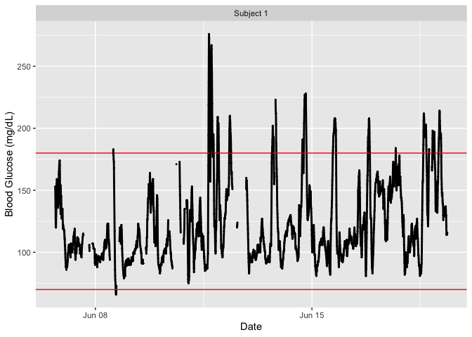
# Summary statistics and some metrics
summary_glu(example_data_1_subject)
#> # A tibble: 1 × 7
#> # Groups:   id [1]
#>   id         Min. `1st Qu.` Median  Mean `3rd Qu.`  Max.
#>   <fct>     <dbl>     <dbl>  <dbl> <dbl>     <dbl> <dbl>
#> 1 Subject 1    66        99    112  124.       143   276

in_range_percent(example_data_1_subject)
#> # A tibble: 1 × 3
#>   id        in_range_63_140 in_range_70_180
#>   <fct>               <dbl>           <dbl>
#> 1 Subject 1            73.9            91.7

above_percent(example_data_1_subject, targets = c(80,140,200,250))
#> # A tibble: 1 × 5
#>   id        above_140 above_200 above_250 above_80
#>   <fct>         <dbl>     <dbl>     <dbl>    <dbl>
#> 1 Subject 1      26.1      3.40     0.377     99.3

j_index(example_data_1_subject)
#> # A tibble: 1 × 2
#>   id        J_index
#>   <fct>       <dbl>
#> 1 Subject 1    24.6

conga(example_data_1_subject)
#> # A tibble: 1 × 2
#>   id        CONGA
#>   <fct>     <dbl>
#> 1 Subject 1  37.0

# Load multiple subject data
data(example_data_5_subject)

plot_glu(example_data_5_subject, plottype = 'lasagna', datatype = 'average')
#> Warning: Removed 5 rows containing missing values or values outside the scale range
#> (`geom_tile()`).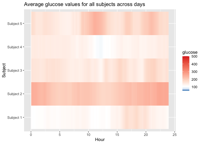
below_percent(example_data_5_subject, targets = c(80,170,260))
#> # A tibble: 5 × 4
#>   id        below_170 below_260 below_80
#>   <fct>         <dbl>     <dbl>    <dbl>
#> 1 Subject 1      89.3      99.7    0.583
#> 2 Subject 2      16.8      78.4    0
#> 3 Subject 3      72.7      95.9    0.848
#> 4 Subject 4      91.0     100      1.69
#> 5 Subject 5      54.6      90.1    1.03

mage(example_data_5_subject)
#> Gap found in data for subject id: Subject 2, that exceeds 12 hours.
#> # A tibble: 5 × 2
#> # Rowwise:
#>   id         MAGE
#>   <fct>     <dbl>
#> 1 Subject 1  72.4
#> 2 Subject 2 118.
#> 3 Subject 3 116.
#> 4 Subject 4  70.9
#> 5 Subject 5 142.
Shiny App
Shiny App can be accessed locally via
or globally at https://irinagain.shinyapps.io/shiny_iglu/. As new functionality gets added, local version will be slightly ahead of the global one.